
Introduction
Machine learning has become an integral part of various industries by allowing computers to learn from data and make predictions or decisions without explicit programming. Linear regression, a fundamental algorithm in machine learning, is widely used in fields such as finance, economics, and psychology to understand and predict the behavior of variables. For example, linear regression can be used to analyze the relationship between a company's stock price and its earnings or predict the future value of a currency based on its past performance.
Linear Regression Fundamentals
Linear regression is a statistical modeling technique that aims to find the relationship between a dependent variable and one or more independent variables. It assumes a linear relationship and creates a linear equation that best fits the given data points. This equation is then used to predict outcomes based on new input data.
To illustrate, let's consider a dataset that includes information about house prices based on their sizes. The dataset has two columns: "Size" (in square feet) and "Price" (in thousands of dollars).
| Size (in sqft) | Price (in $1000 USD) |
|---|---|
| 1000 | 250 |
| 1500 | 400 |
| 2000 | 450 |
| 2500 | 500 |
| 3000 | 550 |
By visualizing the data points on a scatter plot, we can observe a positive linear relationship between the size of houses and their prices.
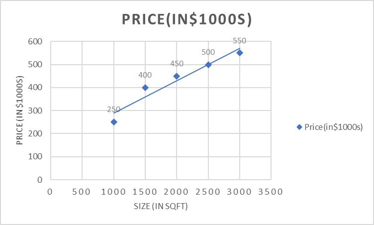
Linear regression performs the task to predict a dependent variable value (y) based on a given independent variable (x)). In the figure above, X (input) is the size of the house and Y (output) is the price of the house. The regression line is the best-fit line for the model.
Types of Linear Regression
Simple Linear Regression
Simple linear regression is the most basic form of linear regression. It involves a single independent variable (often referred to as "x") and the dependent variable ("y"). The goal is to find a linear relationship between the independent and dependent variables. The equation of a simple linear regression model can be represented as:
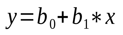
where y is the dependent variable, x is the independent variable, b 0 is the y-intercept, and b 1 is the coefficient for x, also known as the slope.
Multiple Linear Regression
Multiple linear regression extends the concept of simple linear regression by considering multiple independent variables to predict the dependent variable. The equation for a multiple linear regression model can be represented as:
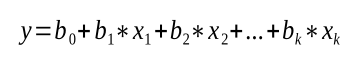
where x 1 , x 2 , ..., x k are the independent variables, and b 1 , b 2 , ..., b k are the corresponding coefficients. Multiple linear regression allows for more sophisticated models that incorporate multiple factors that influence the dependent variable.
Polynomial Regression
Polynomial regression is a variation of linear regression where the relationship between the independent and dependent variables is approximated using polynomial functions. It allows for modeling non-linear relationships by introducing polynomial terms of the independent variables, such as squared terms (x 2 ), cubed terms (x 3 ), or higher-order terms.
The equation for a polynomial regression model can be represented as:
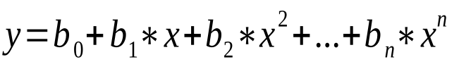
where n represents the degree of the polynomial.
Other Variations and Techniques
- Ridge Regression: Incorporates regularization to handle multicollinearity (high correlation) among independent variables.
- Lasso Regression: Uses regularization and also performs feature selection by shrinking some irrelevant features to zero, effectively removing them from the model.
- Elastic Net Regression: Combines the techniques of ridge and lasso regression, offering a balance between regularization and feature selection.
- Logistic Regression: A type of generalized linear regression used for predicting binary or categorical outcomes by applying a logistic function to the linear equation.
Known Algorithms
XGBoost Algorithm
XGBoost stands for “Extreme Gradient Boosting”. It is an optimized distributed gradient boosting library designed for efficient and scalable training of machine learning models. It is an ensemble learning method that combines the predictions of multiple weak models to produce a stronger prediction which means that they build a model by sequentially adding weak learners (such as decision trees) to improve the overall performance of the model.
XGBoost can handle large datasets and achieve state-of-the-art performance in many machine learning tasks such as classification and regression. It has built-in support for parallel processing, making it possible to train models on large datasets in a reasonable amount of time.
CatBoost Algorithm
CatBoost or Categorical Boosting is an open-source boosting library developed by Yandex. It is designed for use on problems like regression and classification having a very large number of independent features.
Catboost is a variant of gradient boosting that can handle both categorical and numerical features. It does not require any feature encodings techniques like One-Hot Encoder or Label Encoder to convert categorical features into numerical features.
Linear Learner Algorithm on linear regression
Linear models are supervised learning algorithms used for solving either classification or regression problems. For input, you give the model labeled examples ( x , y ). x is a high-dimensional vector and y is a numeric label. The algorithm learns a linear function, or, for classification problems, a linear threshold function, and maps a vector x to an approximation of the label y.
K-Nearest Neighbors (k-NN) Algorithm
The k-nearest neighbors algorithm, also known as KNN or k-NN, is a non-parametric, supervised learning classifier, which uses proximity to make classifications or predictions about the grouping of an individual data point. It is a popular Machine Learning algorithm used mostly for solving classification problems.
The K-NN algorithm compares a new data entry to the values in a given data set (with different classes or categories). Based on its closeness or similarities in a given range ( K) of neighbors, the algorithm assigns the new data to a class or category in the data set (training data).
Comparing the Algorithms
| Model | Type | Assumptions | Advantages | Disadvantages |
|---|---|---|---|---|
| XGBoost | Gradient boosting | None | Very powerful and accurate, can handle nonlinear relationships and missing data | Can be computationally expensive to train, hyperparameters can be difficult to tune |
| CatBoost | Gradient boosting | None | Similar to XGBoost, but has some advantages such as better performance on categorical data and faster training times | Similar to XGBoost |
| Linear learning | Parametric | Linear relationship between target and independent variables | Simple to understand and implement, interpretable results | Can only capture linear relationships, can be sensitive to outliers |
| KNN | Non-parametric | None | Simple to understand and implement, can handle non-linear relationships | Can be computationally expensive for large datasets, sensitive to outliers |
Performance Assessment
Several metrics are used to assess the performance of regression models and determine how well the fitted line captures the data pattern
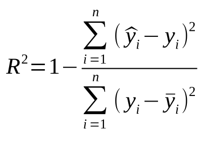
R-squared (R 2 ) Score:
R-squared is a statistical measure that represents the proportion of the variance in the dependent variable (y) that is predictable from the independent variables (x) in the model. It ranges from 0 to 1, with a higher value indicating a better fit.
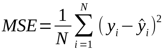
Mean Squared Error (MSE):
MSE is one of the most widely used metrics for evaluating regression models. It measures the average squared difference between the predicted values and the actual values in the dataset. Lower MSE values indicate better model performance.
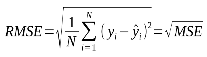
Root Mean Squared Error (RMSE):
RMSE is derived from MSE by taking the square root of the mean squared error. It gives us an estimate of the average absolute difference between the predicted and actual values. Like MSE, lower RMSE values indicate better model performance.
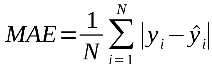
Mean Absolute Error (MAE):
MAE calculates the average absolute difference between the predicted and actual values. It provides a direct measure of the prediction errors, regardless of their directions (positive or negative). Smaller MAE values mean better model performance.
Adjusted R-squared:
Adjusted R-squared is an adjusted version of the R-squared score that penalizes adding unnecessary predictors to the model.
Residual Analysis:
Residual analysis involves examining the differences between the actual and predicted values (residuals) to assess the goodness of fit.
Conclusion
Linear regression is a versatile algorithm in the field of machine learning, offering various techniques to analyze and predict relationships between variables. Understanding the different types of linear regression and performance assessment metrics is crucial for developing accurate and reliable regression models.